Student Name

Capella University

RSCH-FPX7864 Quantitative Design and Analysis

Professor Name

Submission Date

Descriptive Statistics

Part 1: Histogram

Figure 1

Lower Division

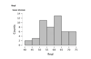
All of the lower-division student grades at the end of their exams have been plotted in a histogram. Histograms are among the most useful and readily available tools for investigating a data set and for discovering patterns in that data, according to Shreffler & Huecker (2023). The exam scores of lower division students are aligned with respect to the number of students who received a grade within each 5- point range between 40 and 75 points. The most frequent score numerically is between 60 and 65 (13 students). The overall frequency distribution is negatively skewed; that is a greater number of students have a score less than the median score of about 60, compared with students who have a score higher than the median score of about 60. The left-skewed frequency distribution shows that most of the scores are more common in the higher levels of the scoring categories and only become less common as scores get lower in the scoring categories.

Figure 2

Upper Division

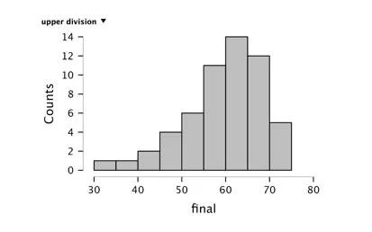
The histogram represents 5-point intervals from 30 to 80 and the number of students who scored on the final exam. The two variables shown in the histogram are the independent variable, the final exam score, and the dependent variable, the upper division classification of a student. The intervals are therefore set up to make it easy to determine the hierarchy among students’ performance and, at the same time, evaluate the number of students included in each interval. Sixty-five to 70 was the interval with the highest number of students sampled (14 students). Histograms are a very effective visual format and widely used in various disciplines to show the distribution of a number of incidents over a range of possible values of a variable, as mentioned by Scheer et al. (2022). The histogram has a bell-shaped, symmetrical distribution, suggesting that the data distribution closely resembles the normal distribution.

Part 02: Descriptive Statistics

Table 1

Descriptive Statistics

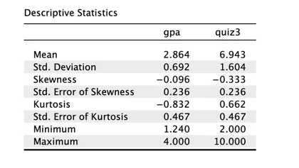
Descriptive statistics such as mean, standard deviation, skewness, and kurtosis are key in establishing the trends of data distribution and central elements of a data set. Descriptive statistics give an overview of the data and the main features of the sample (Fulk, 2023). The closer the mean and the SD are to each other, the closer the data will be to the mean, and the bigger the difference between the mean and SD, the bigger the difference between the spread of the data. In the case of the GPA variable, the average and standard deviation were M = 2.864, SD = 0.692, respectively. The total value of the values is 3.556, which gives a high level of concentration and high central tendency. The values obtained in the Quiz 3 variable are: M = 6.943 and SD = 1.604, and the highest value is 8.547, also indicating concentrated values and a high centrality level. Skew and kurtosis are other measures of normality in the distribution of descriptive statistics, in addition to the central tendency (Hatem et al., 2022). The skew value of the GPA variable was determined to be -0.096, and the Kurtosis was -0.832, both of which are within acceptable limits of -2 and +2, and therefore are normally distributed. On the same note, Quiz 3 variable gave out skewness and kurtosis of -0.333 and 0.662, respectively, all of which lie well within the acceptable boundaries of normality.

Conclusion

Descriptive statistics were used to analyse the frequencies and measures of central tendency of the two groups of students. The first-year students showed a negative skew, and the upper or second-year students were more nearly normal and peaked between 65 and 70. The data for both variables were normally distributed enough to be demonstrated by mean, standard deviation, skewness, and kurtosis values; none of which were outside the range of -2 to +2 as defined for skewness and kurtosis, providing additional support to the assertion that both variables were approximately centered at their means and were normally distributed.